A real-time controller for a home battery
Using a 15 minute battery plan inside a house that changes every few seconds
Battery
MILP
Dynamic Programming
In the previous post I described a 15 minute battery planner. It takes prices, forecasts, battery limits, and the current state of charge, then solves for a cheap battery schedule.
That is a useful planning problem. It is also too slow to be the whole controller.
A house does not behave in 15 minute blocks. A kettle runs for two minutes. Clouds pass. A heat pump cycles. The smart meter can move from import to export and back again several times inside one planning interval.
This post is about the layer underneath the planner. The planner still thinks in 15 minute periods. The real-time controller thinks in seconds.
The main idea is simple. The 15 minute optimiser should not only tell the battery what it planned to do. It should tell the real-time controller what stored energy is worth.
Then the fast controller can decide whether a live meter event is worth spending battery energy on.
Why this gets harder after saldering
Until the end of 2026, Dutch households and small businesses can still use the salderingsregeling. Exported solar can be netted against imported electricity. From January 1, 2027, that ends. The Dutch government explains the change here: Rijksoverheid, salderingsregeling.
Before 2027, the battery problem is often close to a pure timing problem. Charge when power is cheap. Discharge when power is expensive. The exact split between local solar use and grid export is less important, because netting makes import and export partly fungible over the bill.
After 2027, import and export become separate economic events.
\[ \lambda^{buy}_t \neq \lambda^{sell}_t \]
Usually:
\[ \lambda^{buy}_t > \lambda^{sell}_t \]
An imported kWh includes taxes and supplier costs. An exported kWh receives a lower compensation. A kWh used directly inside the house is worth more than a kWh sent to the grid.
That makes the live house state matter. If the battery discharges while the house has no load, it may simply export stored energy at a low price. If the battery charges during a cloud, it may cause extra import. If the battery fills before a sunny afternoon, it may leave no room for solar.
The planner still matters. It knows the day-ahead prices and the forecast. But it cannot see every kettle, cloud, and heat pump cycle.
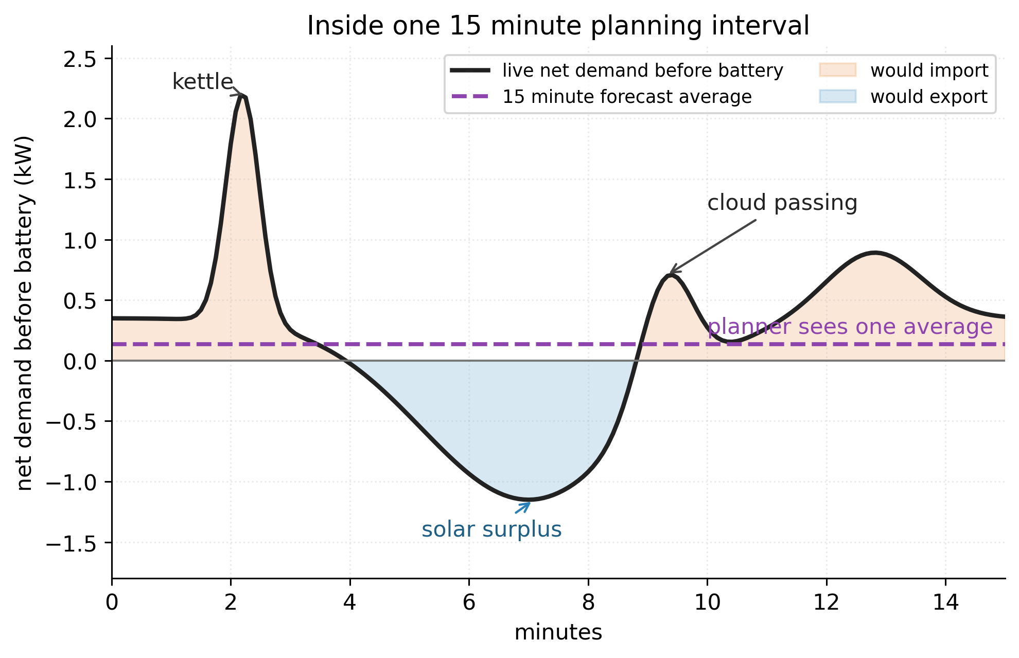
What happens inside one 15 minute period
Take one planning interval. The optimiser has one forecast load value and one forecast PV value for that whole interval, or perhaps one average value. The house has a different reality.
For example, in the same 15 minutes:
- the forecast says 0.5 kW net load;
- the first five minutes have 1.0 kW import;
- the next five minutes have 1.5 kW PV surplus;
- the last five minutes have a 2.5 kW cooking spike.
The 15 minute average can be right while the second-by-second behaviour is very different.
That is the awkward part. The battery plan is made on averages. The smart meter records what actually happened. A 15 minute average close to zero can still contain paid imports and low-value exports inside the interval.
There are two simple controllers one might try.
The first follows the battery plan strictly. If the plan says charge at 800 W, it charges at 800 W. If the plan says discharge at 800 W, it discharges at 800 W.
That is easy to reason about, but it ignores the live meter. It may charge from the grid when the forecast expected solar. It may discharge into export when the forecast expected load.
The second controller is zero on meter. It charges whenever the house would export and discharges whenever the house would import.
That works well for self-consumption. It reacts to real load and real solar. But it is short-sighted. It can empty the battery on a modest afternoon import and leave nothing for the evening peak. It can also fill the battery before a period where empty capacity would be more valuable.
The better controller needs both pieces of information:
- the live meter state;
- the future value of stored energy or empty space.
The live meter comes from the house. The future value comes from the optimiser.
The useful output of the optimiser
The optimiser already returns a schedule:
\[ P^{ch,*}_t,\quad P^{dis,*}_t,\quad E^*_t \]
Those are useful. They show what the planner expected.
But for the fast controller, the most useful output is a value curve.
Let:
\[ V_{t+1}(E) \]
be the future profit from the next 15 minute boundary onward, if the battery starts that future period with energy \(E\).
This curve answers a practical question.
If I end this 15 minute period with 6 kWh in the battery instead of 5 kWh, how much better or worse is that?
The slope of the curve is the marginal value of stored energy:
\[ \pi_{t+1}(E) = \frac{dV_{t+1}}{dE} \]
If \(\pi(E)\) is high, stored energy is valuable. The controller should be careful about discharging.
If \(\pi(E)\) is low, stored energy is not very valuable. The controller can use the battery more freely.
If \(\pi(E)\) is negative, empty space is valuable. This can happen before negative prices or before a sunny period where exporting has low or negative value. A full battery is then a liability.
This is the bridge between the 15 minute optimiser and the real-time controller.
The plan says what looked best under the forecast. The value curve says what battery energy is worth if reality moves away from that forecast.
One sign convention matters. The value curve above is written as future profit. If the planning model minimizes future cost \(J(E)\), then use:
\[ V(E) = -J(E) \]
The slope of \(V\) is then the value of stored energy. Using the slope of \(J\) directly would flip the signs.
Estimating the value curve
If the planning problem is a linear program, the solver can often give dual values. The dual of the initial battery energy constraint is the marginal value of one more kWh.
If the planning problem is a MILP, the dual values are less clean. A simple method is to solve the future planning problem several times with different initial battery energies.
Note that we don’t have to consider a very wide range of initial battery energies, because inside the 15 minute window, we can only charge or discharge the battery by \(\frac{1}{4} P_{\text{battery}}\) kWh.
To estimate our value curve we can for example solve the planning problem for
\[ E_{\text{init,perturbed}} \in \{E_{\text{init}}-\frac{1}{4} P_{\text{battery}}, E_{\text{init}}-\frac{1}{8} P_{\text{battery}}, E_{\text{init}}+\frac{1}{8} P_{\text{battery}}, E_{\text{init}}+\frac{1}{4} P_{\text{battery}}\}\text{ kWh} \]
For each value, solve the future problem and record the optimal profit:
\[ V(E) \]
This gives sampled points. The controller can then use a smoothed interpolation of those points.
There is one catch. A MILP can produce a jagged curve. Binary variables can make one sampled point look oddly bad or oddly good. The raw slope can jump around.
A cleaner control signal is often the upper concave envelope of the sampled points.
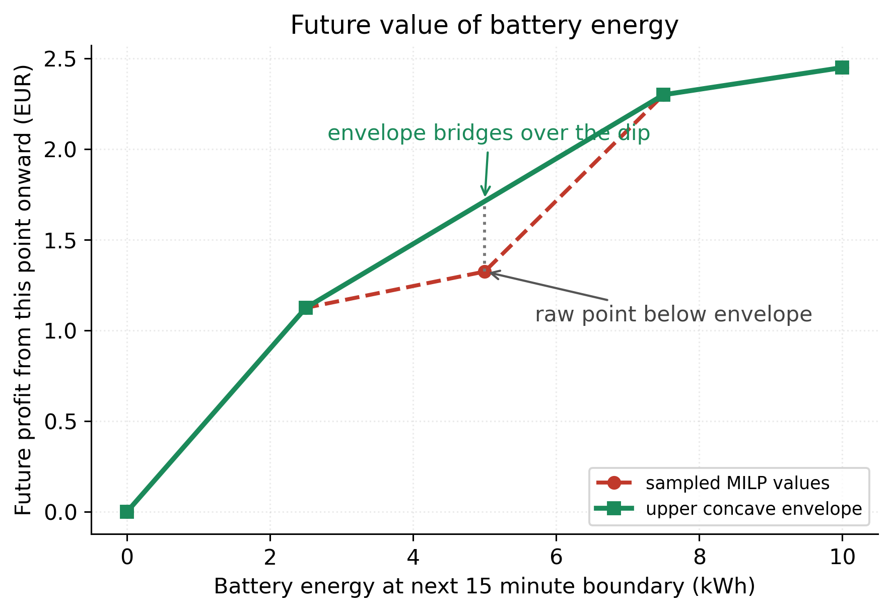
A concave curve has slopes that fall as you move to the right. This is the usual diminishing returns shape. The first kWh in an empty battery may be very valuable. The last kWh in a nearly full battery may be less valuable.
The curve does not always have to slope upward. If empty capacity is valuable, the slope can be negative. The important thing is that the slope should not jump up and down without reason.
For a MILP, the concave envelope is not guaranteed to be the exact value function. It is a regularised value signal for the fast controller. It removes local integer artefacts that would otherwise make the real-time controller twitchy.
That is a tradeoff. If the binary threshold is economically real, smoothing may hide some detail. The practical test is backtesting. Compare the raw sampled curve, the concave envelope, and a simple LP-derived value curve against historical load and PV data.
The derivative is what the real-time controller uses.
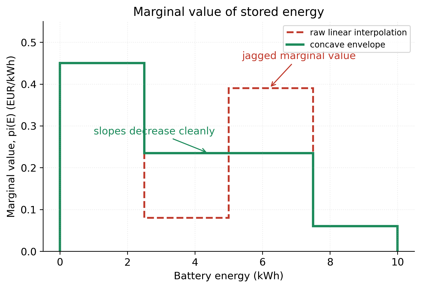
The raw interpolation in the example has marginal values that go down, then up, then down again. A fast controller using that signal may behave strangely near the jump.
The concave envelope gives a cleaner sequence of marginal values. It says: stored energy is very valuable when the battery is low, less valuable in the middle, and least valuable near the top.
That is easier to control.
The real-time decision
Use a signed battery power convention:
\[ p > 0 \]
means discharging.
\[ p < 0 \]
means charging.
Let:
\[ n = P^{load} - P^{pv} \]
be the live site demand before battery action.
If \(n > 0\), the house has a deficit and would import.
If \(n < 0\), the house has surplus and would export.
After battery action, grid power is:
\[ g = n - p \]
Positive \(g\) is import. Negative \(g\) is export.
Every few seconds, the controller asks whether charging or discharging is worth it.
For a deficit, discharging avoids import. Discharge if the import price is higher than the future value of the stored energy, adjusted for losses and wear:
\[ \lambda^{buy} > C^{dis} + \frac{\pi(E)}{\eta^{dis}} \]
For surplus, charging avoids export. Charge if the stored value is higher than the export value, adjusted for losses and wear:
\[ \eta^{ch}\pi(E) > \lambda^{sell} + C^{ch} \]
These two inequalities are the core controller.
They make the battery act like a self-consumption battery when self-consumption is valuable. They also stop it from wasting energy when better use is expected later.
The same logic can allow two active modes.
The battery can charge from the grid when:
\[ \eta^{ch}\pi(E) > \lambda^{buy} + C^{ch} \]
This happens when future stored energy is valuable enough to justify buying electricity now.
The battery can discharge to the grid when:
\[ \lambda^{sell} > C^{dis} + \frac{\pi(E)}{\eta^{dis}} \]
This happens when export is valuable, or when \(\pi(E)\) is negative enough that making empty space is worth it.
Those two modes should be enabled only if the tariff, inverter, and user preference allow them. A conservative controller can start with self-consumption only: charge from local surplus and discharge into local deficit. A more active controller can also use grid charging and export discharge.
The degradation terms are important. The planner may already include battery wear, but the real-time controller still needs to pay for the movement it commands now. Otherwise it will chase tiny meter fluctuations.
The battery should not move unless the value is large enough to pay for losses and wear.
The battery state cannot move that much
Residential batteries are not very fast compared with a 15 minute period.
A 10 kWh battery with a 2.5 kW inverter is a 4 hour battery. At full power, 15 minutes changes the stored energy by:
\[ 2.5 \cdot 0.25 = 0.625 \text{ kWh} \]
That is only 6.25 percent of a 10 kWh battery, before efficiency losses.
This matters because the real-time controller does not need a perfect prediction of the battery energy at the next 15 minute boundary. It needs a good local decision. The loop will run again in a few seconds.
Use a short nowcast, not a full second-by-second forecast system.
Near the current moment, trust the live meter. A few minutes ahead, blend back toward the 15 minute forecast.
A practical nowcast for net site demand before the battery is:
\[ n_{\text{now}} \approx P^{grid}_{\text{now}} + P^{batt}_{\text{now}} \]
where positive means the house would import without the battery.
For the next few minutes, use a filtered version of that number. Farther into the interval, blend back to the planner forecast:
\[ \hat n(\tau) = w(\tau)n_{\text{now,filtered}} + (1-w(\tau))n_{\text{forecast}} \]
Close to now, \(w(\tau)\) is near 1. Toward the next 15 minute boundary, \(w(\tau)\) falls.
This is not a perfect forecast. It is not supposed to be. It is a way to avoid treating a two minute kettle spike as if it lasts for the rest of the planning interval.
A small short-horizon version
The threshold rule is often enough. A slightly better version is a tiny short-horizon controller inside the current 15 minute period.
At minute 5, there are 10 minutes left. The controller can simulate a few candidate battery powers over the next short step, use a nowcast for the next few minutes, and add the terminal value at the 15 minute boundary.
The problem is:
\[ \max_{p_0,\ldots,p_{N-1}} \sum_{i=0}^{N-1} r_i(g_i,p_i) + V_{t+1}(E_N) \]
subject to the battery dynamics and limits.
Only the first setpoint is applied. A few seconds later, the calculation is repeated.
This sounds more complicated than it is. The battery power is one-dimensional. A home controller can evaluate a small grid of candidate powers, such as:
\[ \{-P^{max},\ldots,0,\ldots,P^{max}\} \]
and choose the best allowed value.
The first version should use the threshold rule. The short-horizon version is worth adding when backtests show that the threshold rule leaves value on the table.
The reason is the 4 hour battery argument. In 5 seconds, or even in 10 minutes, the state cannot move very far. Fresh value curves and sensible guardrails matter more than pretending the within-interval forecast is exact.
What to do with the old battery plan
The real-time controller may look as if it is ignoring the battery plan. That is partly true. It should not blindly track the planned battery power.
The battery plan is a forecast-based path. The real-time controller sees the real house.
The state to protect is not battery power. It is battery energy. Power is a flow. Energy is the stock that carries into the future.
A controller can have very different second-by-second power from the plan and still preserve the plan’s economic purpose, as long as the battery energy remains in a sensible region.
The planned energy path \(E^*_t\) is still useful. It is a diagnostic and a guardrail. If actual energy is far below the planned energy, the value curve may be stale. If actual energy is far above the planned energy, the same may be true.
The clean response is to re-run the planner.
A small correction to the marginal value can be used as a fallback:
\[ \tilde \pi(E) = \pi(E) + k_-(E^* - E)_+ - k_+(E - E^*)_+ \]
If the battery is much emptier than expected, this raises the value of stored energy. If the battery is much fuller than expected, it lowers the value of stored energy.
This correction should not be the main control law. It is a safety measure for the period between planning runs. When the correction becomes large, the planner should run again.
Three controller types
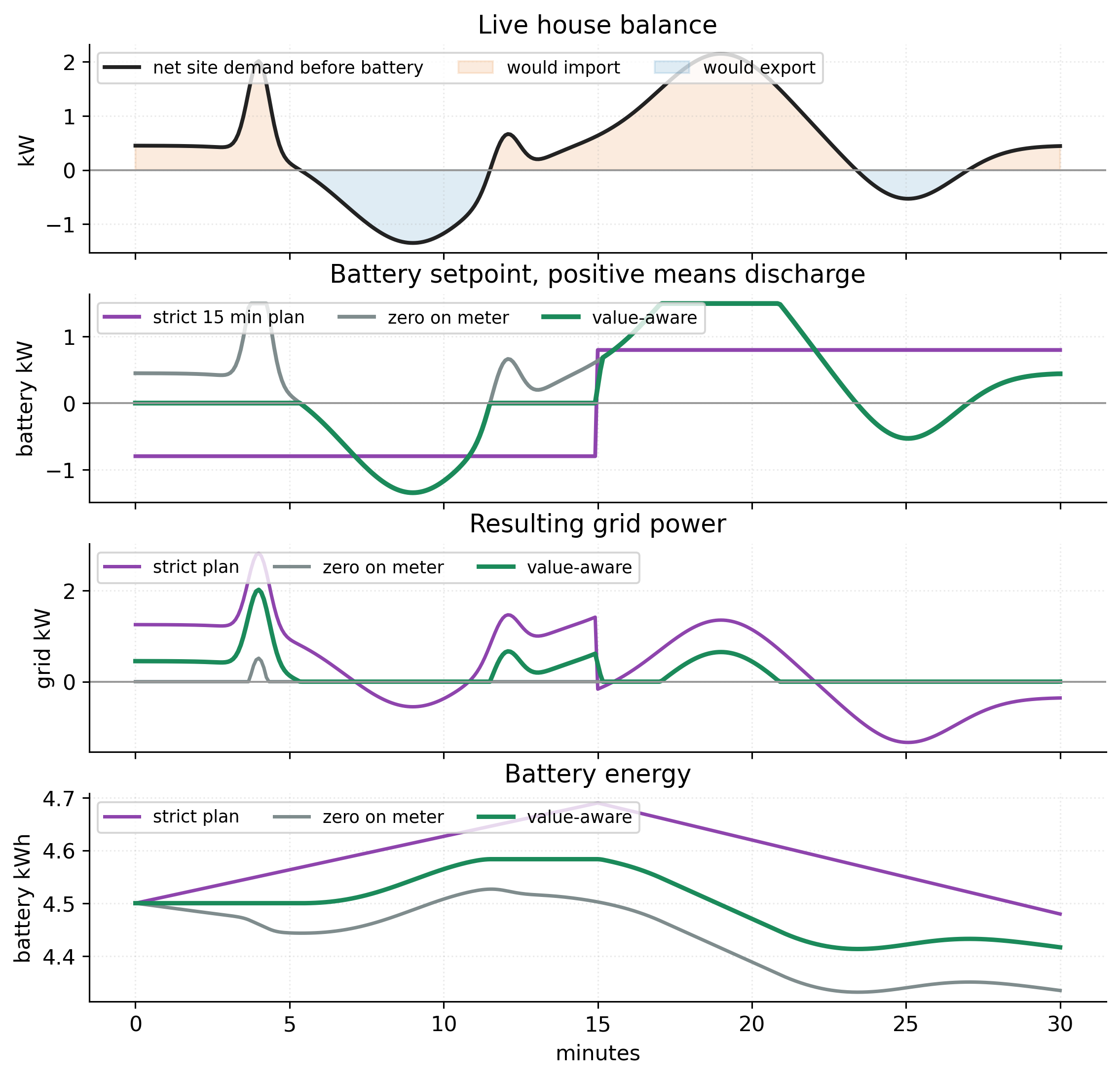
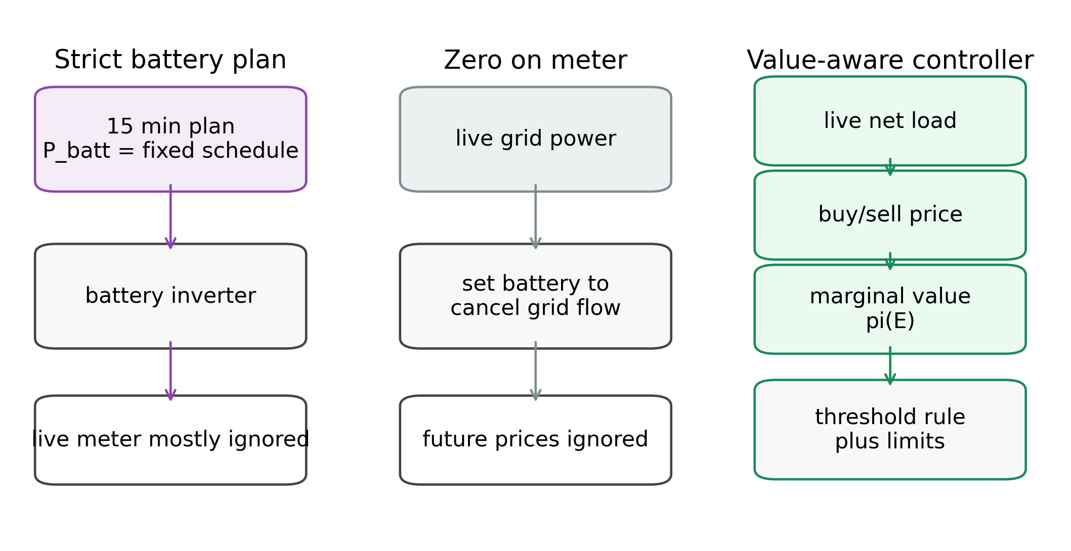
The strict battery plan follows the optimiser’s power setpoint. It is easy to explain but too rigid.
Zero on meter follows the live grid flow. It is fast and useful but blind to the future.
The value-aware controller uses the live meter, the current buy and sell prices, and the marginal value of battery energy from the optimiser.
It does not need a perfect forecast inside the 15 minute window. It needs enough local information to avoid silly actions, and enough long-horizon information to avoid short-sighted ones.
Practical details
A few boring protections make the controller much better.
Filter the live meter signal over 5 to 15 seconds. The battery should respond to real changes, not measurement noise.
Add hysteresis around the thresholds. If discharging becomes attractive at 30 ct/kWh, do not stop again at 29.99 ct/kWh.
Limit setpoint changes. A residential inverter does not need a new command for a 20 W difference.
Use SOC guard bands. If the battery reports 0 to 100 percent, operate inside a narrower range.
Re-run the planner every 15 minutes. Re-run earlier if actual battery energy is far from the planned value, or if the PV forecast is clearly wrong.
Use a fallback. If the optimiser fails or the value curve is stale, fall back to conservative self-consumption or idle mode.
Handle negative export prices explicitly. If exporting costs money, first try to charge the battery or EV. If that is not possible, curtail PV if the inverter allows it.
None of these changes the main idea. They keep the controller from doing fragile things.
The controller in one paragraph
The 15 minute optimiser computes the future value of stored battery energy. The real-time controller reads the live meter every few seconds. If the house is importing, it discharges only when avoiding import is worth more than keeping the energy. If the house has surplus, it charges only when storing that surplus is worth more than exporting it. Losses and degradation create a deadband. The controller does not need a perfect second-by-second forecast, because the battery state moves slowly and the loop keeps repeating.
The slow optimiser thinks about the day. The fast controller thinks about the next few seconds. The value curve is the contract between them.