Predicting Sale Prices Of Houses In Ames
Predicting Sale Prices of Houses in Ames using scikit-learn.
In this tutorial I will discuss how you can go from a raw dataset to a predictive model. For this tutorial we will make use of the Ames Dataset and see whether we can predict house prices based on characteristics provided in the dataset.
The analysis in this tutorial is done in Python using the pandas, scikit-learn and matplotlib packages. We will start by exploring the raw data and see whether we can already see some patterns in the data or that some features should be discarded right away. Next, we will make a straight-forward pipeline that will transform our dataset and fit a linear regression model. Finally, we will evaluate the performance of this model.
I do have limited knowledge with data analysis (I mainly use R), so this tutorial will be most informative for people like me: beginners!
Raw Data & Initial Analysis
First, we need to download the dataset provided in the link above (direct download link here).
import pandas as pd
import numpy as np
import matplotlib.pyplot as plt
from datetime import date
from sklearn.impute import SimpleImputer
from sklearn.preprocessing import LabelBinarizer, StandardScaler, OneHotEncoder
from sklearn.compose import ColumnTransformer
from sklearn.pipeline import make_pipeline
from sklearn.model_selection import train_test_split
from sklearn.linear_model import LinearRegression
import warnings

# Do not display warnings
warnings.filterwarnings('ignore')

# Import the Ames Housing data (put this in the same folder as your Python file)
house_data = pd.read_csv("AmesHousing.txt", sep="\t")

# I do not like spaces in the column names of a dataset so I first replace spaces
# by underscores
house_data.columns = house_data.columns.str.replace(' ', '_')
Next we want to get a feeling for what exactly we can find in the dataset, so let’s look at some relevant information.
# Get some feeling for the data
print(house_data.head(10))
house_info = house_data.describe()
house_data.info()
   Order        PID  MS_SubClass MS_Zoning  Lot_Frontage  Lot_Area Street  \
0      1  526301100           20        RL         141.0     31770   Pave
1      2  526350040           20        RH          80.0     11622   Pave
2      3  526351010           20        RL          81.0     14267   Pave
3      4  526353030           20        RL          93.0     11160   Pave
4      5  527105010           60        RL          74.0     13830   Pave
5      6  527105030           60        RL          78.0      9978   Pave
6      7  527127150          120        RL          41.0      4920   Pave
7      8  527145080          120        RL          43.0      5005   Pave
8      9  527146030          120        RL          39.0      5389   Pave
9     10  527162130           60        RL          60.0      7500   Pave

  Alley Lot_Shape Land_Contour    ...     Pool_Area Pool_QC  Fence  \
0   NaN       IR1          Lvl    ...             0     NaN    NaN
1   NaN       Reg          Lvl    ...             0     NaN  MnPrv
2   NaN       IR1          Lvl    ...             0     NaN    NaN
3   NaN       Reg          Lvl    ...             0     NaN    NaN
4   NaN       IR1          Lvl    ...             0     NaN  MnPrv
5   NaN       IR1          Lvl    ...             0     NaN    NaN
6   NaN       Reg          Lvl    ...             0     NaN    NaN
7   NaN       IR1          HLS    ...             0     NaN    NaN
8   NaN       IR1          Lvl    ...             0     NaN    NaN
9   NaN       Reg          Lvl    ...             0     NaN    NaN

  Misc_Feature Misc_Val Mo_Sold Yr_Sold Sale_Type  Sale_Condition  SalePrice
0          NaN        0       5    2010       WD           Normal     215000
1          NaN        0       6    2010       WD           Normal     105000
2         Gar2    12500       6    2010       WD           Normal     172000
3          NaN        0       4    2010       WD           Normal     244000
4          NaN        0       3    2010       WD           Normal     189900
5          NaN        0       6    2010       WD           Normal     195500
6          NaN        0       4    2010       WD           Normal     213500
7          NaN        0       1    2010       WD           Normal     191500
8          NaN        0       3    2010       WD           Normal     236500
9          NaN        0       6    2010       WD           Normal     189000

[10 rows x 82 columns]
<class 'pandas.core.frame.DataFrame'>
RangeIndex: 2930 entries, 0 to 2929
Data columns (total 82 columns):
Order              2930 non-null int64
PID                2930 non-null int64
MS_SubClass        2930 non-null int64
MS_Zoning          2930 non-null object
Lot_Frontage       2440 non-null float64
Lot_Area           2930 non-null int64
Street             2930 non-null object
Alley              198 non-null object
Lot_Shape          2930 non-null object
Land_Contour       2930 non-null object
Utilities          2930 non-null object
Lot_Config         2930 non-null object
Land_Slope         2930 non-null object
Neighborhood       2930 non-null object
Condition_1        2930 non-null object
Condition_2        2930 non-null object
Bldg_Type          2930 non-null object
House_Style        2930 non-null object
Overall_Qual       2930 non-null int64
Overall_Cond       2930 non-null int64
Year_Built         2930 non-null int64
Year_Remod/Add     2930 non-null int64
Roof_Style         2930 non-null object
Roof_Matl          2930 non-null object
Exterior_1st       2930 non-null object
Exterior_2nd       2930 non-null object
Mas_Vnr_Type       2907 non-null object
Mas_Vnr_Area       2907 non-null float64
Exter_Qual         2930 non-null object
Exter_Cond         2930 non-null object
Foundation         2930 non-null object
Bsmt_Qual          2850 non-null object
Bsmt_Cond          2850 non-null object
Bsmt_Exposure      2847 non-null object
BsmtFin_Type_1     2850 non-null object
BsmtFin_SF_1       2929 non-null float64
BsmtFin_Type_2     2849 non-null object
BsmtFin_SF_2       2929 non-null float64
Bsmt_Unf_SF        2929 non-null float64
Total_Bsmt_SF      2929 non-null float64
Heating            2930 non-null object
Heating_QC         2930 non-null object
Central_Air        2930 non-null object
Electrical         2929 non-null object
1st_Flr_SF         2930 non-null int64
2nd_Flr_SF         2930 non-null int64
Low_Qual_Fin_SF    2930 non-null int64
Gr_Liv_Area        2930 non-null int64
Bsmt_Full_Bath     2928 non-null float64
Bsmt_Half_Bath     2928 non-null float64
Full_Bath          2930 non-null int64
Half_Bath          2930 non-null int64
Bedroom_AbvGr      2930 non-null int64
Kitchen_AbvGr      2930 non-null int64
Kitchen_Qual       2930 non-null object
TotRms_AbvGrd      2930 non-null int64
Functional         2930 non-null object
Fireplaces         2930 non-null int64
Fireplace_Qu       1508 non-null object
Garage_Type        2773 non-null object
Garage_Yr_Blt      2771 non-null float64
Garage_Finish      2771 non-null object
Garage_Cars        2929 non-null float64
Garage_Area        2929 non-null float64
Garage_Qual        2771 non-null object
Garage_Cond        2771 non-null object
Paved_Drive        2930 non-null object
Wood_Deck_SF       2930 non-null int64
Open_Porch_SF      2930 non-null int64
Enclosed_Porch     2930 non-null int64
3Ssn_Porch         2930 non-null int64
Screen_Porch       2930 non-null int64
Pool_Area          2930 non-null int64
Pool_QC            13 non-null object
Fence              572 non-null object
Misc_Feature       106 non-null object
Misc_Val           2930 non-null int64
Mo_Sold            2930 non-null int64
Yr_Sold            2930 non-null int64
Sale_Type          2930 non-null object
Sale_Condition     2930 non-null object
SalePrice          2930 non-null int64
dtypes: float64(11), int64(28), object(43)
memory usage: 1.8+ MB
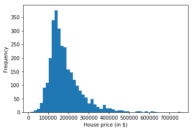
Since we want to build a model that predicts the house price given a set of features of this given house, let’s first check these prices by creating a histogram.
plt.hist(house_data.SalePrice, bins=50)
plt.xlabel("House price (in $)")
plt.ylabel("Frequency")
plt.show()

# Pandas also provides a built-in plotting env
# house_data.SalePrice.plot.hist()
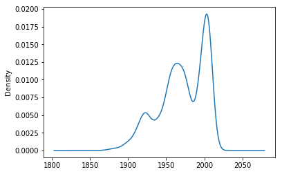
The Year_Built feature would be a candidate to give insights in the sale price of a house. Below we report the density of the year that each house in the dataset is built.
house_data['Year_Built'].plot.kde()
<matplotlib.axes._subplots.AxesSubplot at 0x1a1ab908d0>
We can check the relationship between the sale price and the year houses are built by creating a scatter plot.
house_data.plot.scatter(x='Year_Built', y='SalePrice')
<matplotlib.axes._subplots.AxesSubplot at 0x1a19375160>
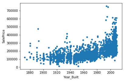
This plot suggest that houses that are built more recently tend to have a higher sale price (on average). Note that this probably due to the geographical area we are considering. In old cities, like Amsterdam, we can imagine that (part) of the old houses are momumental buildings and therefore have higher sale price.
In the analysis above, we have looked into the relationship of the sale price and a numerical feature. A scatter plot is usually a good option to check if there might be an interesting relationship, however for categorical features we need different techniques.
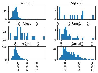
We have information on the type of sale for each house, e.g., some houses are sold with adjecent land, or a family member bought the house. A tool to look at the relationship between this (categorical) feature and the sale price is to look at the histogram for each type of sale condition.
house_data['SalePrice'].hist(by=house_data['Sale_Condition'], bins=30)
array([[<matplotlib.axes._subplots.AxesSubplot object at 0x1a1ad44eb8>,
        <matplotlib.axes._subplots.AxesSubplot object at 0x1a1acd0f98>],
       [<matplotlib.axes._subplots.AxesSubplot object at 0x1a1af29208>,
        <matplotlib.axes._subplots.AxesSubplot object at 0x1a1a944470>],
       [<matplotlib.axes._subplots.AxesSubplot object at 0x1a1ac636d8>,
        <matplotlib.axes._subplots.AxesSubplot object at 0x1a1ae64940>]],
      dtype=object)
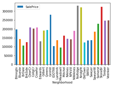
Another feature that is likely to have an influence on the sale price is in what neighbourhood the house is located. We could again create histograms of the sale price for each neighbourhood, but since there are more than 20 neighbourhoods, we can do something else. We take the mean of the sale price for each neighbourhood and present this in a bar plot.
# Check saleprice per neighbourhood
avg_price_neigh = house_data.groupby('Neighborhood').agg({'SalePrice' : 'mean'}).reset_index()
avg_price_neigh.plot.bar(x='Neighborhood', y='SalePrice')
<matplotlib.axes._subplots.AxesSubplot at 0x1a1b026dd8>
Feature Selection
The dataset provides more than 80 features, and not all features are equally informative for sale price. Selecting good features and transforming existing features is often a rather ad-hoc procedure, since every dataset is unique. However, there are a few standard procedures that usually help in creating a significantly better dataset.
Trimming
One of these techniques is to delete outliers from your dataset. Whether or not this is necesarry also depends on the type of model that is used, e.g., linear models are usually very sensitive to outliers.
Let’s look at a scatter plot of the living area and sale price.
# Check living space and sale price (there seems to be 5 outliers...)
house_data.plot.scatter(x='Gr_Liv_Area', y='SalePrice')
house_data = house_data.query('Gr_Liv_Area < 4000')
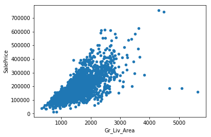
There seem to be 4-5 outliers with very high living areas. For this analysis we will remove these, however if the goal of your model is to also have good predictions for these outliers it might be worthwhile to keep them.
Feature enhancement
There are many ways to enhance existing features. Here, I will show how categorical variables can be improved. To do this, I select all features that are of the type object and save the histogram for these features in a folder figures.
# Check categorical variables and see if we need to delete them
house_data_cat = house_data.select_dtypes(include='object')

for col in house_data_cat.columns:
    house_data_cat[col].value_counts().plot.bar(title=col)
    plt.savefig('figures/' + col + '_hist.pdf')
    plt.clf()

house_data_cat['Bsmt_Qual'].value_counts().plot.bar(title='Basement Quality')
<matplotlib.axes._subplots.AxesSubplot at 0x1a1d629be0>
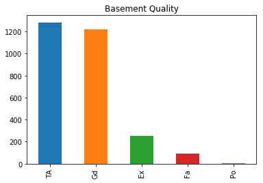
There are a considerable number of categorical features that are ordinal, that is, the categories have a certain ordering. In this case, we have information about whether the feature has a value Poor, Fair, Average, Good or Excellent. However, especially the most extreme outcomes are rather unlikely. As we will later see this results in a large number of features (when we one hot encode them) with only minimal extra predictive power. Therefore we combine certain groups.
ord_groups = {'Fa': 'Bad', 'Po': 'Bad', 'TA': 'Average', 'Gd': 'Good', 'Ex':'Good'}
columns_ord = ['Bsmt_Cond', 'Bsmt_Qual', 'Exter_Cond', 'Exter_Qual', 'Fireplace_Qu',
               'Garage_Cond', 'Garage_Qual', 'Heating_QC', 'Kitchen_Qual', 'Pool_QC']
for col in columns_ord:
    house_data[col].replace(ord_groups, inplace=True)
    house_data[col] = house_data[col].astype('category', categories=['Bad', 'Average', 'Good'], ordered=True)
Missing Values
Most real-life datasets have missing values for a subset of its features. There are different ways to deal with these missing values. Usually, when a feature’s value is missing in most of the samples, it is better to just discard them. Let’s see if we have any of these variables.
missing_vals = house_data.isnull().sum(axis = 0)
print(missing_vals)
Order                0
PID                  0
MS_SubClass          0
MS_Zoning            0
Lot_Frontage       490
Lot_Area             0
Street               0
Alley             2727
Lot_Shape            0
Land_Contour         0
Utilities            0
Lot_Config           0
Land_Slope           0
Neighborhood         0
Condition_1          0
Condition_2          0
Bldg_Type            0
House_Style          0
Overall_Qual         0
Overall_Cond         0
Year_Built           0
Year_Remod/Add       0
Roof_Style           0
Roof_Matl            0
Exterior_1st         0
Exterior_2nd         0
Mas_Vnr_Type        23
Mas_Vnr_Area        23
Exter_Qual           0
Exter_Cond           0
                  ...
Bedroom_AbvGr        0
Kitchen_AbvGr        0
Kitchen_Qual         0
TotRms_AbvGrd        0
Functional           0
Fireplaces           0
Fireplace_Qu      1422
Garage_Type        157
Garage_Yr_Blt      159
Garage_Finish      159
Garage_Cars          1
Garage_Area          1
Garage_Qual        159
Garage_Cond        159
Paved_Drive          0
Wood_Deck_SF         0
Open_Porch_SF        0
Enclosed_Porch       0
3Ssn_Porch           0
Screen_Porch         0
Pool_Area            0
Pool_QC           2914
Fence             2354
Misc_Feature      2820
Misc_Val             0
Mo_Sold              0
Yr_Sold              0
Sale_Type            0
Sale_Condition       0
SalePrice            0
Length: 82, dtype: int64
Let’s get rid of features that have many missing values.
house_data = house_data.drop(columns=['Alley', 'Fireplace_Qu', 'Pool_QC',
                                      'Misc_Feature', 'Misc_Val'])
For some features a missing value is not really missing, since it can indicate that the value of this feature is zero when it’s missing. Fence and Pool_Area belong to this group. For these features we decide to create a binary variable indicating whether or not the house has this feature (and we do not care about the type or size of feature).
# Make some variables useful
house_data['Fence'] = house_data['Fence'].notna()
house_data['Pool'] = house_data['Pool_Area'] > 0
Similar to the categorical features that are rated from poor until excellent, there are also features with different categories. Again, it might be worthwhile to combine categories in the dataset that only occur a very infrequently. In this case we combine categories that consistute less than 1 percent of the total samples.
house_data_obj = house_data.select_dtypes(include='object')
for col in house_data_obj.columns:
    series = house_data[col].value_counts()
    mask = (series/series.sum() * 100).lt(1)
    house_data[col] = np.where(house_data[col].isin(series[mask].index),'Other',
              house_data[col])
    house_data[col] = house_data[col].astype('category')
Note that the 1 percent of the total sample is rather ad-hoc. Imagine that you have a dataset consisting of millions of samples, then there is no need to get rid of these categories, since we still have sufficient information (unless you need balanced categories).
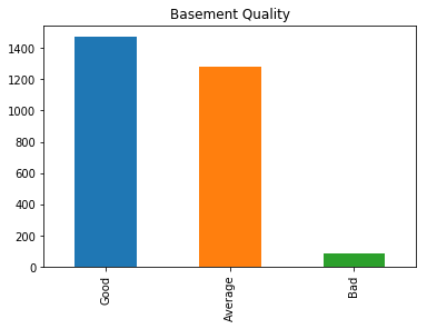
To see what effect our transformations and enhanced have had on our features, we can have a look at the basement quality feature again.
house_data['Bsmt_Qual'].value_counts().plot.bar(title='Basement Quality')
<matplotlib.axes._subplots.AxesSubplot at 0x1a1db4d668>
Data pipeline
Now that we have cleaned and transformed our dataset we can look at if it is possible to create a decent model that can predict sale prices of houses the model has not seen before. However, we first have to deal with a few steps before we can use our dataset in these models.
We need to make sure that we do not evaluate on data that we used to train and estimate our model. So we split our dataset in a training and test part.
X = house_data.drop(columns=['SalePrice'])
y = house_data['SalePrice']

# We need to split the set into a training and test set.
X_train, X_test, y_train, y_test = train_test_split(X, y, test_size=0.2)
Imputer
Even though we got rid of the features with many missing values, there are still features that have a few missing values. It is possible to use advanced techiques to “imputate” these missing values, however we will a simple imputing technique, which replaces the missing values with the most frequent value for that feature.
imputer = SimpleImputer(strategy='most_frequent')
Standardisation & Encoding
Most machine learning models require that the scale of the features in the dataset are similar. Therefore, we will standardise all numerical features in the dataset by removing the mean of that feature and dividing by the standard deviation, i.e.,
We also have categorical features which we cannot directly feed to the machine learning models. All features need to be represented by a numerical value. Both nominal and ordinal features can be transformed by a technique called One-hot encoding, where a categorical feature is replaced by a number of dummies that indicate one of these categories.
# Next we need to scale the numerical columns and encode the categorical
# variables. This can be done by splitting the dataset into two parts.
cat_cols = X_train.select_dtypes(include='category').columns
num_cols = X_train.select_dtypes(include='number').columns

cat_cols_mask = X_train.columns.isin(cat_cols)
num_cols_mask = X_train.columns.isin(num_cols)

ct = ColumnTransformer(
        [('scale', StandardScaler(), num_cols_mask),
         ('encode', OneHotEncoder(), cat_cols_mask)])
Note that ordinal values can also be transformed into a single numerical value, where each category is represented by a number that is ordered according to the ordering of these categories. The advantage of this procedure is that we require less features to represent this feature numerically, however for most machine learning models it also results in a linear relationship between the that feature and the feature we want to predict.
Machine learning model
Now that we have a dataset that only consists of numerical values we can apply any machine learning we want. scikit-learn provides many machine learning models with a common interface (except for the hyperparameters), so it is easy to implement many different models. In our case I will only use a linear regression.
linear_reg = LinearRegression()
Combine all steps of pipeline
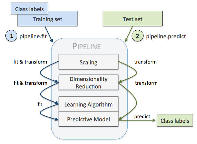
Pipelines can be used to automatically perform all steps of the model estimation (including preprocessing steps). It also makes sure that the preprocessing is done correctly, e.g., the scaling for the test dataset is the one used for the training dataset (Reader: why is this absolutely necessary?). An overview of what the pipeline does is given in the figure below (copyright by Sebastian Raschka).
pipe = make_pipeline(imputer, ct, linear_reg)
Training & Evaluating model
Training the model is as simple as
pipe = pipe.fit(X_train, y_train)
Usually, the best model (within or between) class(es) of models can be determined by using cross-validation or splitting the training dataset into a training and validation part (if you have enough data). I will skip this step and go immediately to the evaluation of our model.
In the step above we estimated and trained our model based on the training set. To see how well it performs we can look at what sale prices our model predict for data it has not seen before.
y_pred = pipe.predict(X_test)
errors = y_pred - y_test
scikit-learn can provide a score for the model, but we will look at the error of the prediction instead. First let’s plot the histogram of the errors
plt.hist(errors, bins=30)
plt.show()
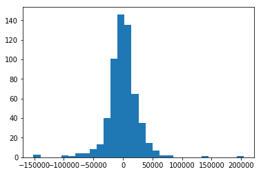
The histogram suggest that the errors are normally distributed (assumption of the linear regression). Furthermore, it seems that most predictions have an error less than 20,000$. To me this seems like a reasonable model.
Conclusion
In this tutorial we have seen how we can go from raw data to a predictive model that has a reasonable performance. However, there are many things we have not discussed yet. To name a few:
- Consider multiple models and select the best one using cross-validation.
- Use a more advanced missing value imputation technique, e.g., MICE.